CausalMGM is a data analysis tool that offers a suite of procedures to quickly explore large, complex datasets. The server produces a graphical model of a dataset where the nodes in the graph correspond to variables in the data, and the edges in the graph depict dependencies among the variables. This allows a user to query their data to 1) find the direct causes of variable(s) of interest, 2) find novel associations between pairs of variables in their data, or 3) identify the best features to develop a predictive model for variable(s) of interest.
If you used CausalMGM in your research, please cite us:
Sedgewick, AJ, Shi, I, Donovan, RM, and Benos, PV. 2016. Learning mixed graphical models with separate sparsity parameters and stability-based model selection. BMC Bioinformatics. 17(S5). p. S175
Sedgewick, AJ, Buschur, K, Shi, I, Ramsey, JD, Raghu, VK, Manatakis, DV, Zhang, Y, Bon, J, Chandra, D, Karoleski, C, Sciurba, FC, Spirtes, P, Glymour, C, and Benos, PV. 2019. Mixed graphical models for integrative causal analysis with application to chronic lung disease diagnosis and prognosis. Bioinformatics. 35(7), pp. 1204-1212.
You may direct questions related to CausalMGM to:
Vineet Kalathur Raghu
E-mail: vkr8@pitt.edu
For question related to CausalMGM Website:
Xiaoyu Ge
E-mail: xig34@pitt.edu
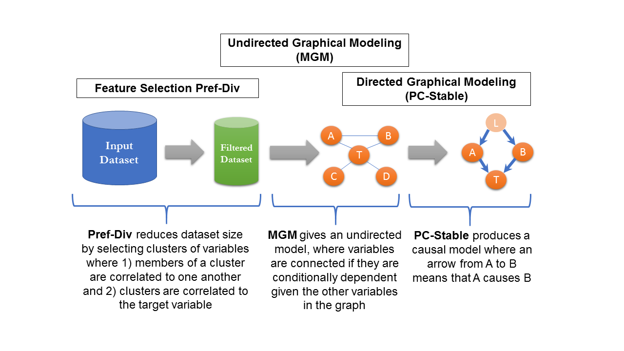
CausalMGM expects a tabular dataset with continuous and categorical variables. It then proceeds in three steps to produce a graphical model of this data: 1) (Optional) Feature selection, 2) Learning an undirected model (a model of associations), 3) (Optional) Learning a directed model (model of cause/effect).
Step 1. Upload the dataset
Some requirements for the dataset are:
Step 2. Configure the experiment
The meaning of each parameter is as follows:
Pref-Div parameters
Number of variables to be selected - This is the number of continuous features to be selected.
hese selected features, the target variable, and all of the categorical variables will be used for graphical modeling. A higher number enables a more accurate graphical model, but will take longer to run and will be more difficult to visualize/interpret.
Name of target variable - Which variable should be treated as the target variable?
Variables to Keep - Comma-separated list of continuous variables that should be automatically included in the final graphical model. (Not counted towards the "number of variables to be selected")
Automatic clustering - Redundant features will be represented as a cluster variable using Principal Component Analysis instead of a single representative of the entire cluster.
Graphical Modeling Parameters
Lambda parameters determine the sparsity level of the mixed graphical model. A higher lambda value results in fewer (but higher confidence) edges in the output graph. There are separate lambda parameters for each edge type.
Lambda 1 - Controls sparsity for edges between two continuous variables.
Lambda 2 - Controls sparsity for edges between continuous and categorical variables.
Lambda 3 - Controls sparsity for edges between two categorical variables.
Lambda values can be automatically chosen based on stability using the "Find Lambdas" button. Note that this operation can be time consuming for large datasets.
Alpha - PC-Stable requires an alpha value. This is the p-value threshold for the conditional independence tests. A lower alpha value means a sparser graph because fewer tests will meet the threshold for significance.
Some requirements for the dataset are:
- Must be in tabular format with variable names in the first row.
- Must have no missing data.
- Must contain only continuous and categorical variables (no censoring).
- Ordinal variables will be treated as continuous if there are more than 5 categories.
- To treat these as categorical, combine categories to reduce the number to 5.
- To treat these as continuous, use real numbered values (e.g. 2.0, 3.0, etc.).
- You can use the Check my Data button to confirm proper format
Step 2. Configure the experiment
The meaning of each parameter is as follows:
Pref-Div parameters
Number of variables to be selected - This is the number of continuous features to be selected.
hese selected features, the target variable, and all of the categorical variables will be used for graphical modeling. A higher number enables a more accurate graphical model, but will take longer to run and will be more difficult to visualize/interpret.
Name of target variable - Which variable should be treated as the target variable?
Variables to Keep - Comma-separated list of continuous variables that should be automatically included in the final graphical model. (Not counted towards the "number of variables to be selected")
Automatic clustering - Redundant features will be represented as a cluster variable using Principal Component Analysis instead of a single representative of the entire cluster.
Graphical Modeling Parameters
Lambda parameters determine the sparsity level of the mixed graphical model. A higher lambda value results in fewer (but higher confidence) edges in the output graph. There are separate lambda parameters for each edge type.
Lambda 1 - Controls sparsity for edges between two continuous variables.
Lambda 2 - Controls sparsity for edges between continuous and categorical variables.
Lambda 3 - Controls sparsity for edges between two categorical variables.
Lambda values can be automatically chosen based on stability using the "Find Lambdas" button. Note that this operation can be time consuming for large datasets.
Alpha - PC-Stable requires an alpha value. This is the p-value threshold for the conditional independence tests. A lower alpha value means a sparser graph because fewer tests will meet the threshold for significance.
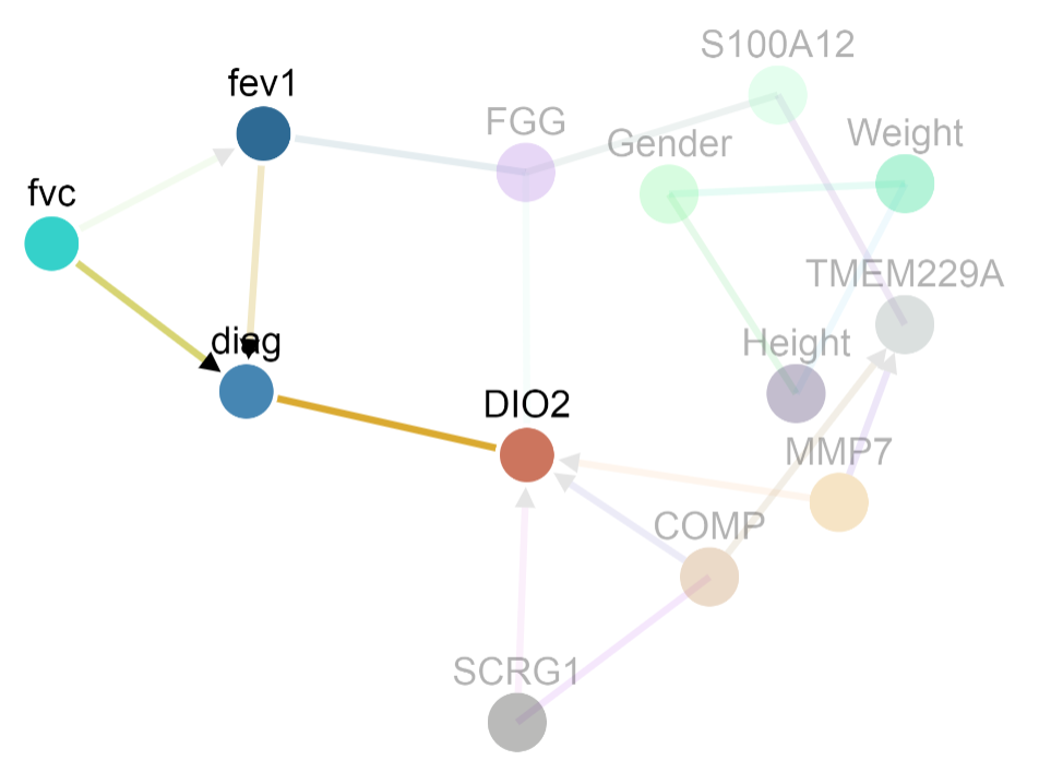
The sample dataset comes from a population with two lung conditions: 1) Idiopathic Pulmonary Fibrosis (IPF) and 2) Chronic Obstructive Pulmonary Disorder (COPD). The goal was to identify factors that distinguish IPF from COPD.
Undirected model
For the undirected model below, gender is connected to only height and weight. This means that 1) the best variables to predict gender in this dataset are height and weight and 2) gender is conditionally dependent on height (and weight) given the rest of the variables in the graph. In an undirected model, an edge between A and B could arise because of any of the four conditions:
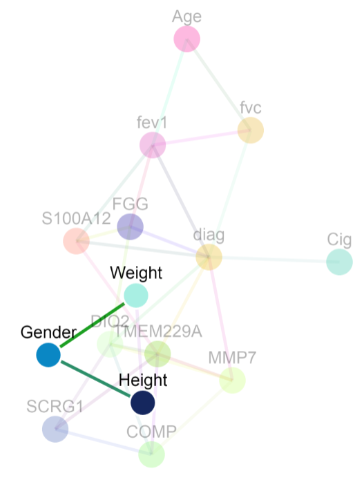
- A causes B
- B causes A
- A and B are both controlled by a confounder
- A and B are associated because of selection bias for the data sample
- Datasets larger than 1000 variables should use feature selection prior to running, otherwise computations may take a very long time.
- Censored data and data with missing values will not work.
- Interactions between continuous variables are assumed to be linear and these variables must be close to normally distributed.
- Interpreting directed edges as causal requires additional assumptions including: no cycles in the graph, no latent confounders.